Swin Transformer 论文阅读笔记
论文来源:
【ICCV 2021 最佳论文】 Swin Transformer: Hierarchical Vision Transformer Using Shifted Windows [Paper] [Code]
研究动机和思路
“We seek to expand the applicability of Transformer such that it can serve as a general-purpose backbone for computer vision, as it does for NLP and as CNNs do in vision.” 我们试图扩展 Transformer 的适用性,使其可以作为计算机视觉任务的通用主干,就像它在 NLP 领域和 CNN 在视觉邻域中所起到的效果。
图像信息建模:如下图所示,
ViT在对图像进行自注意力时,始终在原图1/16大小的patch上进行,实现图像信息的全局建模。受限于此,**ViT无法从局部层面提取图像特征,以及无法实现图像多尺度特征的表示**(在密集预测型任务中尤为重要,如图像分割和目标检测)。
时间复杂度:由于标准
Transformer架构的自注意力计算过程是在token和token之间进行,因此复杂度极大程度上取决于token的数量。
“The global computation leads to quadratic complexity with respect to the number of tokens.” 全局计算复杂度是关于 token 数量的二次复杂度。
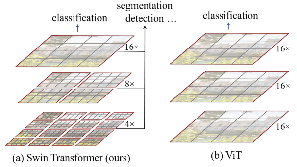
如何兼顾局部和全局
Swin Transformer 的实现方式:
(1)预处理:将输入图像取成4×4 (pixel)的小patch;
(2)Layer L:使用7×7 (patch)的window将patch块圈起来,在该window内对7×7=49个patch进行自注意力,实现图像局部特征的建模;
(3)Layer L+1:通过滑动window使得原本不在一个window内的patch处于一个window内,通过对其进行自注意力实现cross-window connections。
(4)通过步长为s的patch merging将临近的 小 patch 合并成patch, 使得整图分辨率下降1/s,实现多尺度图像特征的提取;
(5)当图像尺寸减少至一定程度时,一个window能够对整图进行处理,实现图像全局特征的建模。
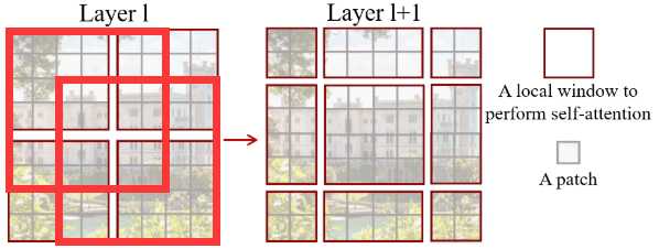 shifted window approach shifted window approach |
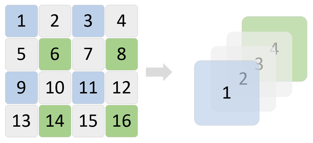 patch merging(序号仅用于理解) patch merging(序号仅用于理解) |
Swin Transformer
网络架构
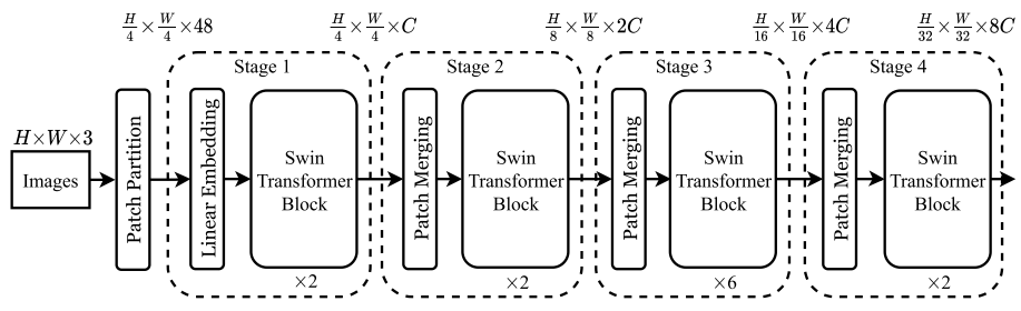
以下结合网络架构图和代码推导一下(阅读文字时可将代码块折叠) 👇👇👇:
注:区别于 ViT 的一点在于,Swin Transformer 在进行分类任务时没用引入 class token,而是在最后使用 global average pooling (GAP) 得到类别预测的结果,目的在于使得 Swin Transformer 能够很好地兼容到视觉的其他任务中,如图像分割和目标检测。
Patch Embedding
Patch Partition:不妨设输入图像尺寸为 ${H}\times{W}\times{C_{in}}$,
Swin Transformer将patch size设置为 ${4}\times{4}$,则一个token的大小为 ${4}\times{4}\times{C_{in}}$,token序列的长度为 $\frac{H}{4}\times\frac{W}{4}$;因此,整幅图像被转化成了维度为 $(\frac{H}{4}\times\frac{W}{4})\times({4}\times{4}\times{C_{in}})$ 的token序列,以224×224×3的输入图像为例,其产生的token序列的长度为(56×56)×(16×16×3);(以上过程通过4×4卷积层实现)
Linear Embedding:通过
Patch Partition得到的token序列的长度对于Transformer模型而言是巨大的,因此需要减少其长度至设定的超参数 $C$;(以上过程通过Linear层实现)
1 | |
Hierarchical Stage
以
stage2为例(stage3、4同理),推导一下网络:
(1)Layer Input:输入特征图维度为 $\frac{H}{4}\times\frac{W}{4}\times{C}$;
(2)Patch Merging:经上图右侧所示过程,合并 patch 之后的特征图尺寸减少1/2倍,通道数增加4倍,即经patch merging之后的输出特征图维度为 $\frac{H}{8}\times\frac{W}{8}\times{4C}$;
(3)Channel Reduction:为了保持与卷积神经网络拥有相同的层级表示,进一步通过Linear层或1×1卷积层(二者作用一致,原文代码用的Linear层)将通道数降为2C,使得最终输出特征图维度为 $\frac{H}{8}\times\frac{W}{8}\times{2C}$;(注:本过程为Patch Merging中的步骤)
(3)Swin Transformer Block:
1 | |
Swin Transformer Block
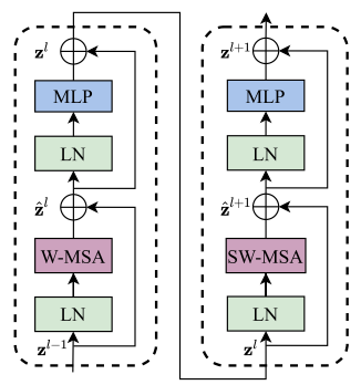
Shifted Window based Multi-head Self-Attention
前面提到,Swin Transformer 通过设置 window,对处于 window 内的 patch 做自注意力。以 stage1 为例,56×56 的 patch 数量,设置 7×7 的 window size,对整图运算则需要的 window 数量为 (56/7)×(56/7)=8×8=64。
计算复杂度分析
(1)标准Multi-head Self-attention:
$$3HWC^{2}+(HW)^{2}C+(HW)^{2}C+HWC^{2}=4HWC^{2}+2(HW)^{2}C, \tag{1}$$
(2)Swin Transformer中的Self-attention:
$$(\frac{H}{M}\times\frac{W}{M})\times(4MMC^{2}+2(MM)^{2}C)=4HWC^{2}+2M^{2}HWC, \tag{2}$$
将 $(2)$ 式减 $(1)$ 式得 $(HW-M^{2})\times(2HWC)$,确实有 一定程度 的下降。