图像投影网络(Image Projection Network, IPN)系列论文阅读笔记
主要是以下两篇论文:
IPN(TMI 2020):Image Projection Network: 3D to 2D Image Segmentation in OCTA Images
IPN V2(arXiv 2020):IPN-V2 and OCTA-500: Methodology and Dataset for Retinal Image Segmentation
图像投影网络的设计来源
眼科临床
“Comparing to color fundus imaging technology, OCT can acquire more detailed information about retinal structures and thus becomes a leading modality in the clinic observation of retinopathy.” 与彩色眼底成像技术相比,OCT可以获取更详细的视网膜结构信息,成为视网膜病变临床观察的主要方式。
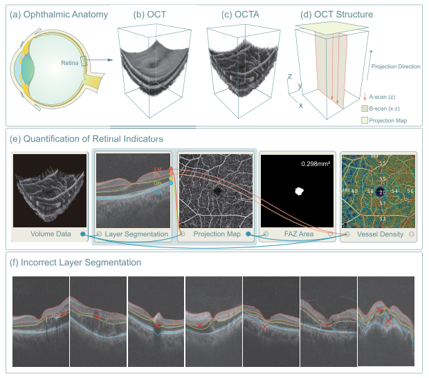
诊疗指标
“Both OCT and OCTA can provide 3D data, but most retinal indicators, such as the vessel density and the FAZ area, are quantified on the projection maps rather than 3D space.” OCT 和 OCTA 都可以提供 3D 数据,但大多数视网膜指标,例如血管密度和 FAZ 面积,都是在投影图(上图 e)上量化的,而不是在 3D 空间上。
数据标注问题
对于医生而言,在 OCT 或 OCTA 的 3D 数据上直接进行标注是困难的,相反在 2D 的投影图上标注则是相对简单和高效的。
已有深度学习方法的的局限性
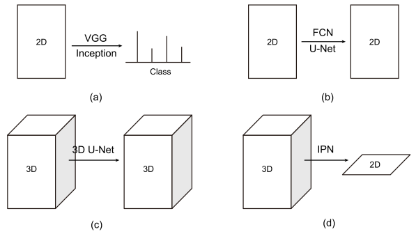
主流端到端方法:
(1)2D to category.
(2)2D to 2D semantic segmentation.
(3)3D to 3D semantic segmentation.
对于(3)而言,应用到 OCT 和 OCTA 图像上是几乎不可能的:
“Alternatively, they need 3D pixel-to-pixel labels, which are labor-intensive and difficult to be obtained.” 或者,他们需要 3D 像素到像素的标签,这是劳动密集型且难以获得的。
Image Projection Network (IPN)
2D-to-1D IPN
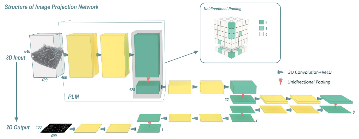
(1)构造方式:
“We use the framework of the classical VGG model for reference, remove all the full connection layers, and change the original pooling layer to the unidirectional pooling layer.” 我们借鉴经典VGG模型的框架,去掉所有的全连接层,将原来的池化层改为单向池化层(下图右)。
(2)实现方式:
将3×400×640的横截面图输入上述构造的IPN中,输出得到一维的尺寸为1×400×1的向量;通过将每个病例的400张横截面图像输入网络得到的输出向量拼接,即可得到1×400×400的预测图像。
(3)局限性:
最终的分割结果是通过拼接得到的,由于包含很多锯齿状的边缘,空间连续性较差。

3D-to-2D IPN
“IPN can summarize the effective features in 3D data along the projection direction and output the segmentation results on a 2D plane, to realize the semantic segmentation from 3D to 2D.” IPN 可以沿投影方向总结 3D 数据中的有效特征并在 2D 平面上输出分割结果,实现从 3D 到 2D 的语义分割。
与 2D-to-1D IPN 的差异:使用 3D 卷积 而不是 2D 卷积,并且单向池化从 2D 扩展到 3D,但仍然只作用在投影方向。 通过这种变化,IPN 可以输入 3 维图像并输出 2 维截面图。以下介绍 3D-to-2D IPN 的关键组成部分。
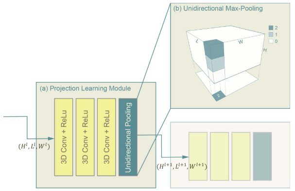
投影学习模块
Projection Learning Module, PLM
(1)组成部分:三个 卷积核尺寸为(3×3×3)的 3D 卷积层和一个单向池化层。
(2)单个PLM的输入输出尺寸变化:$[H \times L \times W] \rightarrow [\frac{H}{k} \times L \times W]$,其中k为单向池化层的pooling size。
模型架构
| Layer | Channel Number | PLM Parameter | Output Size |
| Input | 2 | - | 640×100×100 |
| PLM1 | 32 | 5 | 128×100×100 |
| PLM2 | 64 | 4 | 32×100×100 |
| PLM3 | 128 | 4 | 8×100×100 |
| PLM4 | 256 | 4 | 2×100×100 |
| PLM5 | 512 | 2 | 1×100×100 |
| Conv6 | 256 | - | 1×100×100 |
| Conv7 | 128 | - | 1×100×100 |
| Conv8 | 2 | - | 1×100×100 |
| Softmax | 2 | - | 1×100×100 |
代码实现
以下实现时,为了适应后面 IPN V2 论文中的输入,做了一些改动:
(1)输入 Patch 大小为 640×100×100;
(2)减少一个 pooling size = 4 的 PLM 层,以适应输出;
(3)减少最后的卷积层至 1 层;
(4)将Softmax替换成了Sigmoid,训练过程中的损失函数使用BCELoss(),而非原文中提到的CELoss(),本质是一样的。
1 | |
1 | |
训练细节
RV Segmentation
输入数据:3D 的 OCT 和 OCTA Volume,原始数据大小为 640px × 400px × 400px;
输入大小:640px × 100px × 100px 的采样数据;
采样方式:由于投影图中血管分布均匀,因此采用 随机采样。
FAZ Segmentation
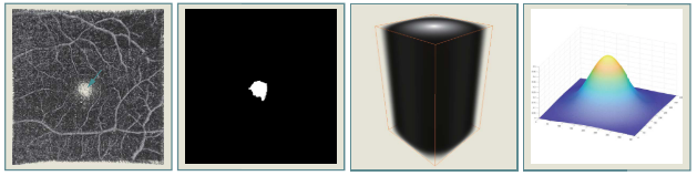
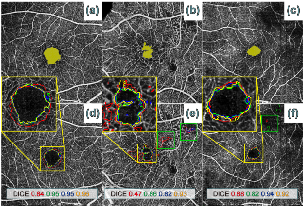
输入数据:除了 3D 的 OCT 和 OCTA Volume外,还考虑到 FAZ 位于图像的中心区域,添加了下图所示的距离图(distance map)作为第三通道;
输入大小:640px × 100px × 100px 的采样数据;
采样方式:由于投影图中 FAZ 仅占一小部分,导致 FAZ 的分割中存在正负样本的不平衡问题,为了增加正样本的比例,采用以投影中心为中心的 正态分布采样,以增加中心位置被选为训练数据的概率。
参数配置
| Optimizer | Adam Stochastic Optimization |
| GPU | 1 NVIDIA GeForce GTX 1080Ti |
| Loss Function | Cross-entropy |
| Batch Size | 3 |
| Max Iteration Number | 20000 |
| Initial Learning Rate | 10^(-4) |
对比实验
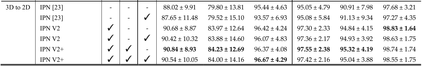
3D-to-2D IPN vs. 2D-to-1D IPN
2D-to-1D IPN 在训练过程中缺少空间信息,导致预测结果中心存在明显的锯齿状。

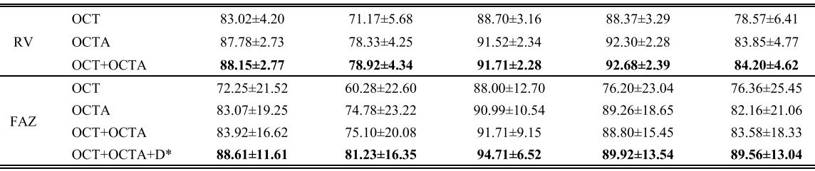
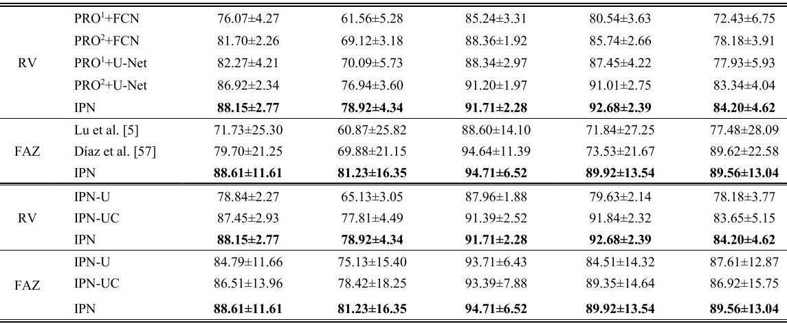
Multi-Channel vs. Single-Channel
(1)OCTA > OCT;
(2)多模态数据 > 单模态数据;
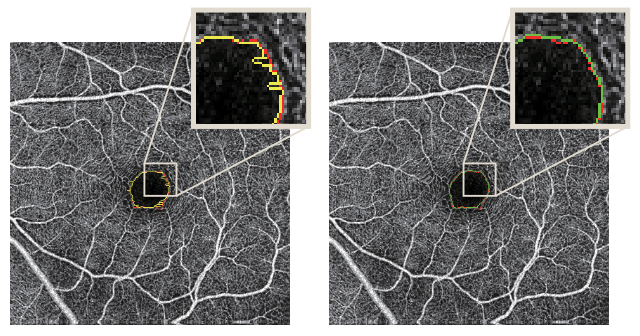
(3)Distance Map 的引入 增大了中心区域的权重,使得 FAZ 的分割结果上涨了 5 个百分点。(”Distance map plays an important role, which is related to the location specificity of FAZ. Without the distance map, the network mistakenly assumes that the areas with weak blood flow signals belong to FAZ, such as the weakening of local signals due to turbid refractive media and non-perfusion zone.” 距离图起着重要的作用,这与 FAZ 的位置特异性有关。 在没有距离图的情况下,网络错误地认为血流信号较弱的区域属于FAZ,例如由于屈光介质混浊和非灌注区导致局部信号减弱。)
IPN vs. Others
(1)IPN 优于任何 2D 方法
(2)IPN 架构优于 U-Net 架构(max-pooling 和 skip-connection)
IPN V2
Plane Perceptron
设计 V2 版本的出发点:IPN 的主要功能是将 3D 体积信息汇总成 2D 平面。 由于缺乏水平方向的下采样,它缺乏二维平面中的高级语义信息。
解决方法:使用 U-Net 作为平面感知器(Plane Perceptron),并将其连接在 IPN 后面。 此外,将 IPN 输出的 2D 特征和第一个 PLM 输出的 3D 特征连接起来,以防止梯度消失并加快收敛进程。
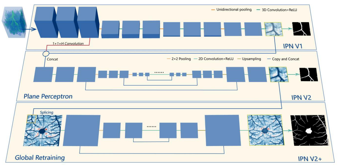
Global Retraining
简单来说,就是把 IPN V2 的预测结果(Patch)拼接到一起,然后再用 U-Net 训练一遍。 并且,在图像拼接的时候采用 重叠 的方法以减少拼接过程带来的“棋盘效应”。
训练细节
IPN V2 的训练细节较 IPN 而言有较大变化:
(1)数据集扩充:从 316 例 6mm×6mm,扩充至 300 例 6mm×6mm 和 200 例 3mm×3mm 的 OCT 和 OCTA Volume;原始数据大小分别为 640px × 400px × 400px 和 640px × 304px × 304px;
(2)输入大小:分别为 160px × 100px × 100px 和 160px × 76px × 76px 的采样数据;
(3)参数调整:Maximum iteration number - 30000,Batch size - 1;
(4)Global Training 参数:Maximum iteration number - 5000,Batch size - 2。
对比实验
RV Segmentation
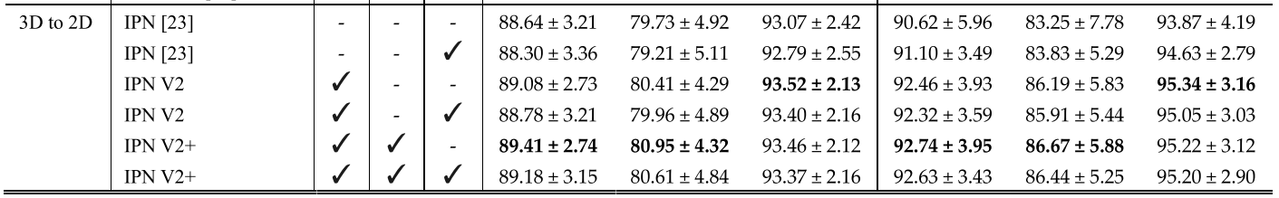
FAZ Segmentation